Os question paper

Questions paper :  Download now

unit-1

1.

2.

3).

4).

5)

unit-2

1).

  A process is a program in execution and it is an active entity. Program counter always specifies address of the next instruction to execute in the next process. Sometimes many processes associate with one program.

Process State :

As a process executes, it changes state. The state of a process is defined by means of  the current activity. The following are the various  states of the process.

i) new:  The process is being created.

ii) running:  Instructions are being executed.

iii) waiting:  The process is waiting for some event to occur.

iv) ready:  The process is waiting to be assigned to a process.

v) terminated:  The process has finished execution

2). 

Process Control Block (PCB) :

Each process is represented in operating system by a process control block or task control block. The PCB contains the following information associated with each process.

i) Process state

ii) Program counter

iii) CPU registers

iv) CPU scheduling information

v) Memory-management information

vi) Accounting information

vii) I/O status information

Process No. : It contains identification of process.

Process State : It contains information about state of the process. The entry in the in this state may be new / ready / running / waiting / terminated.

Pointers or CPU Scheduling information : This information contains pointers to various scheduling queues. Pointers to some other processes, process priority etc.,

Program Counter : It contains address of the next instruction to be executed in the process.

Registers : Each process requires to use various registers like accumulator, index register, stacks and general purpose registers. These registers are used to store information regarding process switching. The following diagram shows the concept of process switching and usage of registers.

I/O information : This information inputs various I/O devices allocated to this process, list of open files etc.,

Accounting Information : This information includes amount of  CPU time required for the process, memory required for the process etc.

4).

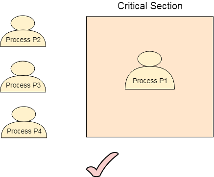
The Critical Section Problem

Critical Section is the part of a program which tries to access shared resources. That resource may be any resource in a computer like a memory location, Data structure, CPU or any IO device.

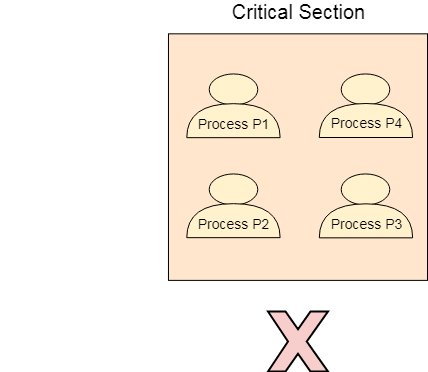
The critical section cannot be executed by more than one process at the same time; operating system faces the difficulties in allowing and disallowing the processes from entering the critical section.

The critical section problem is used to design a set of protocols which can ensure that the Race condition among the processes will never arise.

In order to synchronize the cooperative processes, our main task is to solve the critical section problem. We need to provide a solution in such a way that the following conditions can be satisfied.

Requirements of Synchronization mechanisms

Primary

1. Mutual Exclusion

Our solution must provide mutual exclusion. By Mutual Exclusion, we mean that if one process is executing inside critical section then the other process must not enter in the critical section.






2. Progress

Progress means that if one process doesn't need to execute into critical section then it should not stop other processes to get into the critical section.

Secondary

1. Bounded Waiting

We should be able to predict the waiting time for every process to get into the critical section. The process must not be endlessly waiting for getting into the critical section.

2. Architectural Neutrality

Our mechanism must be architectural natural. It means that if our solution is working fine on one architecture then it should also run on the other ones as well

Peterson’s solution provides a good algorithmic description of solving the critical-section problem and illustrates some of the complexities involved in designing software that addresses the requirements of mutual exclusion, progress, and bounded waiting.

do {
   flag[i] = true;
   turn = j;
   while (flag[j] && turn == j);
   /* critical section */
   flag[i] = false;
   /* remainder section */
}
while (true);

The structure of process Pi in Peterson’s solution. This solution is restricted to two processes that alternate execution between their critical sections and remainder sections. The processes are numbered P0 and P1. We use Pj for convenience to denote the other process when Pi is present; that is, j equals 1 − I, Peterson’s solution requires the two processes to share two data items −

Disadvantage

• Peterson’s solution works for two processes, but this solution is best scheme in user mode for critical section.

• This solution is also a busy waiting solution so CPU time is wasted. So that “SPIN LOCK” problem can come. And this problem can come in any of the busy waiting solution.

5). 

 Semaphores are integer variables that are used to solve the critical section problem by using two atomic operations, wait and signal that are used for process synchronization.

The definitions of wait and signal are as follows −

• Wait

  The wait operation decrements the value of its argument S, if it is positive. If S is negative or zero, then no operation is performed.

wait(S)
{
   while (S<=0);

   S--;
}

• Signal

  The signal operation increments the value of its argument S.

signal(S)
{
   S++;
}

Types of Semaphores

There are two main types of semaphores i.e. counting semaphores and binary semaphores. Details about these are given as follows −

• Counting Semaphores

  These are integer value semaphores and have an unrestricted value domain. These semaphores are used to coordinate the resource access, where the semaphore count is the number of available resources. If the resources are added, semaphore count automatically incremented and if the resources are removed, the count is decremented.

• Binary Semaphores

  The binary semaphores are like counting semaphores but their value is restricted to 0 and 1. The wait operation only works when the semaphore is 1 and the signal operation succeeds when semaphore is 0. It is sometimes easier to implement binary semaphores than counting semaphores.

Advantages of Semaphores

Some of the advantages of semaphores are as follows −

• Semaphores allow only one process into the critical section. They follow the mutual exclusion principle strictly and are much more efficient than some other methods of synchronization.
• There is no resource wastage because of busy waiting in semaphores as processor time is not wasted unnecessarily to check if a condition is fulfilled to allow a process to access the critical section.
• Semaphores are implemented in the machine independent code of the microkernel. So they are machine independent.

Disadvantages of Semaphores

Some of the disadvantages of semaphores are as follows −

• Semaphores are complicated so the wait and signal operations must be implemented in the correct order to prevent deadlocks.
• Semaphores are impractical for last scale use as their use leads to loss of modularity. This happens because the wait and signal operations prevent the creation of a structured layout for the system.
• Semaphores may lead to a priority inversion where low priority processes may access the critical section first and high priority processes late

Process scheduling is an essential part of a Multiprogramming operating systems. Such operating systems allow more than one process to be loaded into the executable memory at a time and the loaded process shares the CPU using time multiplexing.

3).

Process Scheduling Queues

The OS maintains all PCBs in Process Scheduling Queues. The OS maintains a separate queue for each of the process states and PCBs of all processes in the same execution state are placed in the same queue. When the state of a process is changed, its PCB is unlinked from its current queue and moved to its new state queue.

The Operating System maintains the following important process scheduling queues −

• Job queue − This queue keeps all the processes in the system.

• Ready queue − This queue keeps a set of all processes residing in main memory, ready and waiting to execute. A new process is always put in this queue.

• Device queues − The processes which are blocked due to unavailability of an I/O device constitute this queue.

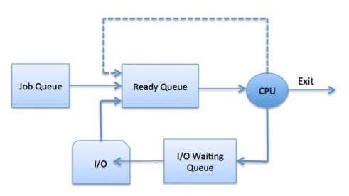
The OS can use different policies to manage each queue (FIFO, Round Robin, Priority, etc.). The OS scheduler determines how to move processes between the ready and run queues which can only have one entry per processor core on the system; in the above diagram, it has been merged with the CPU.

Two-State Process Model

Two-state process model refers to running and non-running states which are described below −

S.N.	State & Description
1	Running When a new process is created, it enters into the system as in the running state.
2	Not Running Processes that are not running are kept in queue, waiting for their turn to execute. Each entry in the queue is a pointer to a particular process. Queue is implemented by using linked list. Use of dispatcher is as follows. When a process is interrupted, that process is transferred in the waiting queue. If the process has completed or aborted, the process is discarded. In either case, the dispatcher then selects a process from the queue to execute.

FCFS Scheduling

First come first serve (FCFS) scheduling algorithm simply schedules the jobs according to their arrival time. The job which comes first in the ready queue will get the CPU first. The lesser the arrival time of the job, the sooner will the job get the CPU. FCFS scheduling may cause the problem of starvation if the burst time of the first process is the longest among all the jobs.

Advantages of FCFS

• Simple
• Easy
• First come, First serv

Disadvantages of FCFS

1. The scheduling method is non preemptive, the process will run to the completion.
2. Due to the non-preemptive nature of the algorithm, the problem of starvation may occur.

Although it is easy to implement, but it is poor in performance since the average waiting time is higher as compare to other scheduling algorithms.

Shortest job first (SJF) or shortest job next, is a scheduling policy that selects the waiting process with the smallest execution time to execute next. SJN is a non-preemptive algorithm. 
 

• Shortest Job first has the advantage of having a minimum average waiting time among all scheduling algorithms.

    It is a Greedy Algorithm.

Round Robin :

Round Robin  is a CPU scheduling algorithm where each process is assigned a fixed time slot in a cyclic way.
 

• It is simple, easy to implement, and starvation-free as all processes get fair share of CPU.
• One of the most commonly used technique in CPU scheduling as a core.
• It is preemptive as processes are assigned CPU only for a fixed slice of time at most.

The disadvantage of it is more overhead of context switching

Priority Based Scheduling

• Priority scheduling is a non-preemptive algorithm and one of the most common scheduling algorithms in batch systems.

• Each process is assigned a priority. Process with highest priority is to be executed first and so on.

• Processes with same priority are executed on first come first served basis.

• Priority can be decided based on memory requirements, time requirements or any other resource requirement.

unit-3

1.Paging is a memory management scheme that eliminates the need for contiguous allocation of physical memory. This scheme permits the physical address space of a process to be non – contiguous.

• Logical Address or Virtual Address (represented in bits): An address generated by the CPU
• Logical Address Space or Virtual Address Space( represented in words or bytes): The set of all logical addresses generated by a program
• Physical Address (represented in bits): An address actually available on memory unit
• Physical Address Space (represented in words or bytes): The set of all physical addresses corresponding to the logical addresses

Example:

• If Logical Address = 31 bit, then Logical Address Space = 231 words = 2 G words (1 G = 230)
• If Logical Address Space = 128 M words = 27 * 220 words, then Logical Address = log2 227 = 27 bits
• If Physical Address = 22 bit, then Physical Address Space = 222 words = 4 M words (1 M = 220)
• If Physical Address Space = 16 M words = 24 * 220 words, then Physical Address = log2 224 = 24 bits

The mapping from virtual to physical address is done by the memory management unit (MMU) which is a hardware device and this mapping is known as paging technique.

• The Physical Address Space is conceptually divided into a number of fixed-size blocks, called frames.
• The Logical address Space is also splitted into fixed-size blocks, called pages.
• Page Size = Frame Size

2.).

Segmentation in Operating System

A process is divided into Segments. The chunks that a program is divided into which are not necessarily all of the same sizes are called segments. Segmentation gives user’s view of the process which paging does not give. Here the user’s view is mapped to physical memory.
There are types of segmentation:

1. Virtual memory segmentation –
   Each process is divided into a number of segments, not all of which are resident at any one point in time.
2. Simple segmentation –
   Each process is divided into a number of segments, all of which are loaded into memory at run time, though not necessarily contiguously.

There is no simple relationship between logical addresses and physical addresses in segmentation. A table stores the information about all such segments and is called Segment Table.

Segment Table – It maps two-dimensional Logical address into one-dimensional Physical address. It’s each table entry has:

• Base Address: It contains the starting physical address where the segments reside in memory.
• Limit: It specifies the length of the segment.\

3) Swapping in Operating System

Swapping is a memory management scheme in which any process can be temporarily swapped from main memory to secondary memory so that the main memory can be made available for other processes. It is used to improve main memory utilization. In secondary memory, the place where the swapped-out process is stored is called swap space.

The purpose of the swapping in operating system is to access the data present in the hard disk and bring it to RAM so that the application programs can use it. The thing to remember is that swapping is used only when data is not present in RAM.

Although the process of swapping affects the performance of the system, it helps to run larger and more than one process. This is the reason why swapping is also referred to as memory compaction.

The concept of swapping has divided into two more concepts: Swap-in and Swap-out.

• Swap-out is a method of removing a process from RAM and adding it to the hard disk.
• Swap-in is a method of removing a program from a hard disk and putting it back into the main memory or RAM.

Example: Suppose the user process's size is 2048KB and is a standard hard disk where swapping has a data transfer rate of 1Mbps. Now we will calculate how long it will take to transfer from main memory to secondary memory.

1. User process size is 2048Kb  
2. Data transfer rate is 1Mbps = 1024 kbps  
3. Time = process size / transfer rate  
4.      = 2048 / 1024  
5.      = 2 seconds  
6.      = 2000 milliseconds  
7. Now taking swap-in and swap-out time, the process will take 4000 milliseconds.   

Advantages of Swapping

1. It helps the CPU to manage multiple processes within a single main memory.
2. It helps to create and use virtual memory.
3. Swapping allows the CPU to perform multiple tasks simultaneously. Therefore, processes do not have to wait very long before they are executed.
4. It improves the main memory utilization.

Disadvantages of Swapping

1. If the computer system loses power, the user may lose all information related to the program in case of substantial swapping activity.
2. If the swapping algorithm is not good, the composite method can increase the number of Page Fault and decrease the overall processing performance.